Exploring Machine Learning in Perspective of Manifold Learning

In this post, I explore machine learning through four fundamental questions, viewed through the lens of manifold learning.

Q1: Why do deep neural networks work so well?

Before deep learning dominated, we relied on traditional methods like SVMs [Cortes & Vapnik, 1995], Random Forests [Breiman, 2001], and simple backpropagation networks [Rumelhart et al., 1986]. These models were small and simple, designed to find direct connections between inputs and outputs.

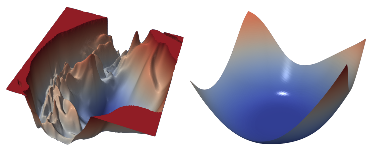
From a manifold learning perspective, the solutions we’re modeling lie on a manifold. Traditional methods worked well for simpler problems (often convex), but struggled with complex tasks like image interpretation where inputs have tens of thousands of dimensions.

Deep neural networks shift us from convex to non-convex optimization—harder to train, but capable of solving remarkably difficult problems in vision, language, and speech.

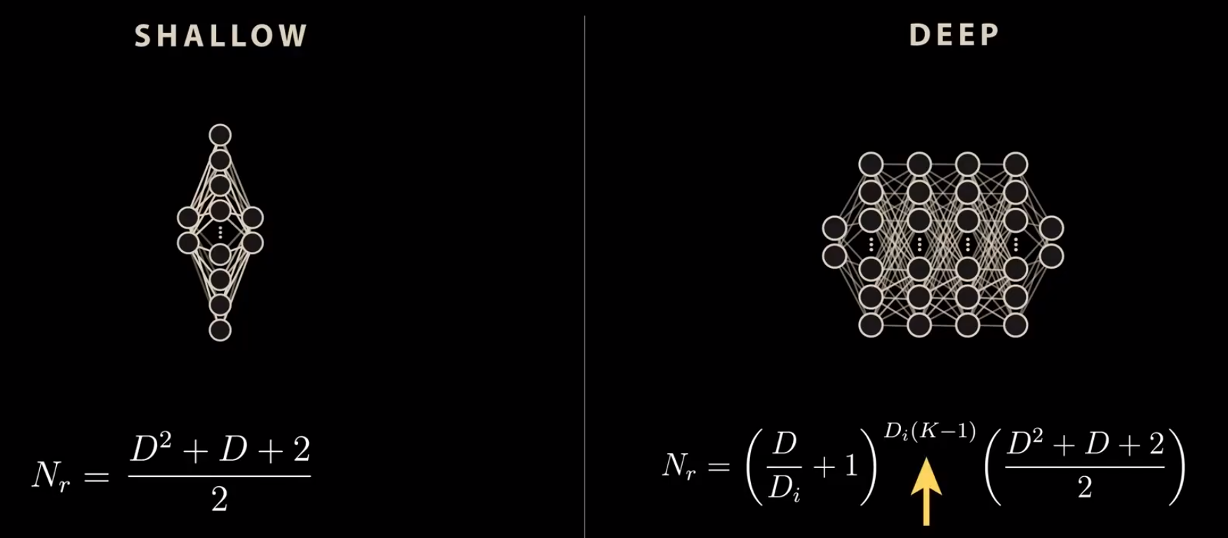
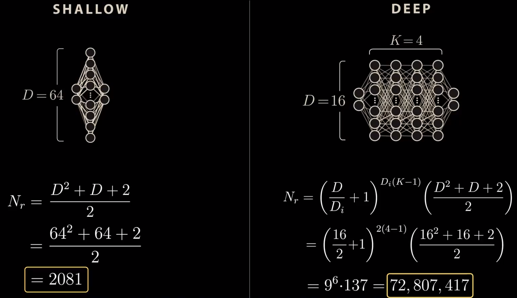
So why do deep neural networks work so well? First (1), the tasks we tackle possess genuine underlying patterns that can be captured by learning algorithms. Second (2), their use of non-linear activation functions—such as ReLU [Nair & Hinton, 2010], GELU [Hendrycks & Gimpel, 2016], SELU [Klambauer et al., 2017], and SwiGLU [Shazeer, 2020]—enables the modeling of complex, non-linear relationships that are otherwise difficult for humans or linear models to capture. Third (3), advances in hardware, notably GPUs, allow for massive parallel computation, making it feasible to train very large models efficiently. Finally (4), deep networks are able to automatically learn hierarchical representations of data, finding effective structures that might be difficult for humans to articulate explicitly.

Another perspective on the success of Deep Neural Networks comes from rethinking generalization. The classical view of the bias-variance trade-off suggests a U-shaped risk curve. However, modern deep learning operates in a regime where high-capacity models continue to generalize well, often described by the “double descent” curve.

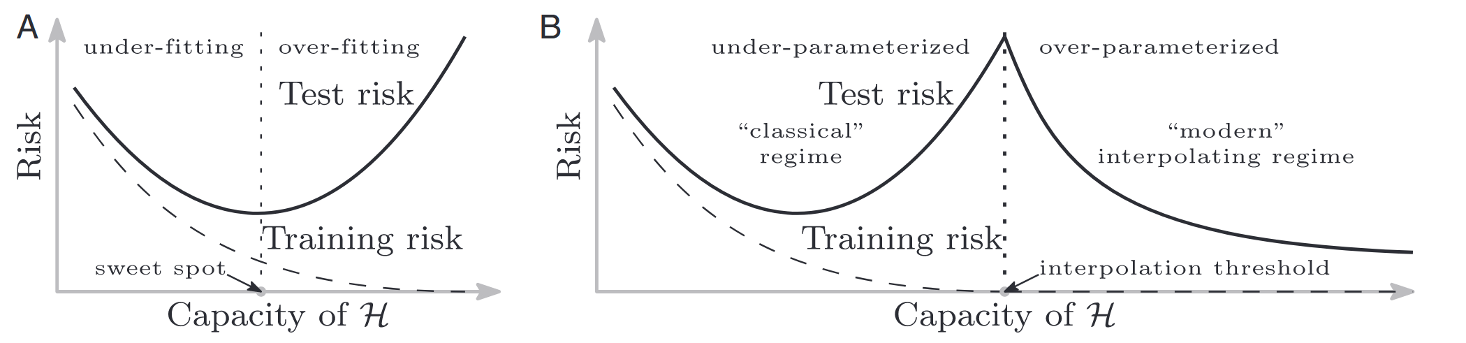
This phenomenon is explored in [Zhang et al., 2017] and [Nakkiran et al., 2020]. It challenges the conventional wisdom that “bigger models are worse” (due to overfitting). Instead, we observe a Double Descent: test error first decreases, then increases (classical overfitting), and then decreases again as the model becomes sufficiently over-parameterized.

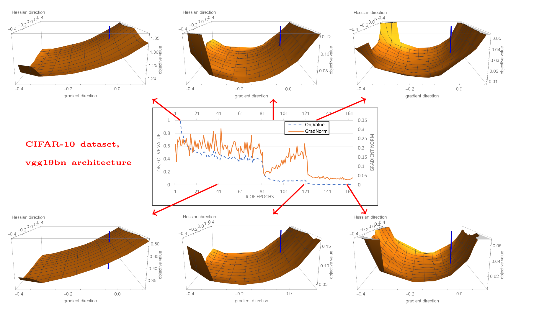
Theoretical works have sought to explain why simple algorithms like SGD can navigate the highly non-convex loss landscapes to find global minima. [Allen-Zhu et al., 2019] provided a convergence theory, showing that for sufficiently wide (over-parameterized) networks, the optimization landscape becomes almost-convex and semi-smooth near random initialization. This guarantees that SGD can find a global minimum (zero training error) in polynomial time.

But convergence to zero training error doesn’t guarantee generalization. This is where Grokking [Power et al., 2022] comes in.

The term “grokking”, originating from Heinlein’s Stranger in a Strange Land, describes a phase transition where a model, long after perfectly overfitting the training set (memorization), suddenly learns to generalize (understanding).

This suggests that “over-training” isn’t just about reaching the bottom of the loss valley, but allowing the model time to “drink” the essence of the structure, moving from a complex memorized solution to a simpler, generalizable one.

Q2: Why state-of-the-art models still show far less generalizability than human beings?

In a recent interview [Sutskever, 2025], Ilya Sutskever highlighted a critical limitation of current AI models:

“The thing which I think is the most fundamental is that these models somehow just generalize dramatically worse than people. It’s super obvious. That seems like a very fundamental thing.”

He suggests that evolution plays a massive role in human sample efficiency by providing a strong “prior” for interacting with the physical world:

“You could actually wonder that one possible explanation for the human sample efficiency that needs to be considered is evolution. Evolution has given us a small amount of the most useful information possible. For things like vision, hearing, and locomotion, I think there’s a pretty strong case that evolution has given us a lot.”

Sutskever contrasts this with machine learning approaches:

• Locomotion: “I mean robots can become dexterous too if you subject them to a huge amount of training in simulation. But to train a robot in the real world to quickly pick up a new skill like a person does seems very out of reach. … So with locomotion, maybe we’ve got some unbelievable prior.”
• Vision: He notes that while children might only practice driving for 10 hours, their visual system is already mature. “I remember myself being a five-year-old… I’m pretty sure my car recognition was more than adequate for driving already… You don’t get to see that much data as a five-year-old… But you could say maybe that’s evolution too.”

However, he distinguishes these evolutionary priors from abstract cognitive skills:

“But in language and math and coding, probably not.”

Q3: Is it possible to build deep neural networks to solve Symbolic Regression?

The short answer is YES! But to understand how, we must first define the challenge.

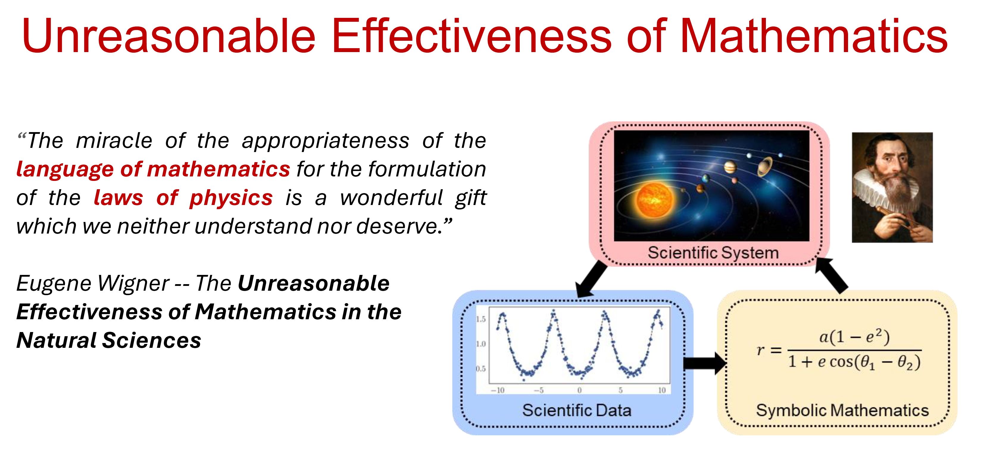
Since the early ages of Natural Sciences in the sixteenth century, the process of scientific discovery has rooted in the formalization of novel insights and intuitions about the natural world into compact symbolic representations of such new acquired knowledge, namely, mathematical equations.

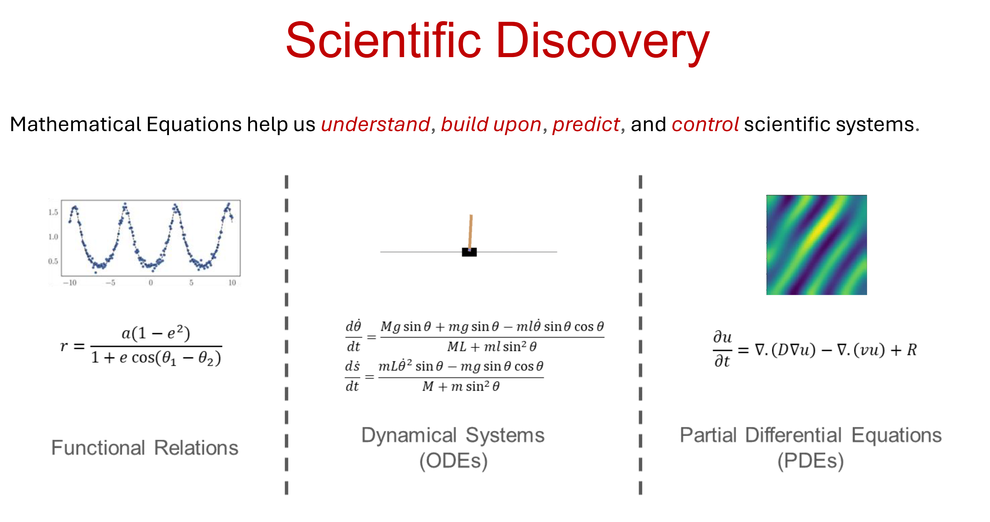
Mathematical equations encode both objective descriptions of experimental data and our inductive biases about the regularity we attribute to natural phenomena.

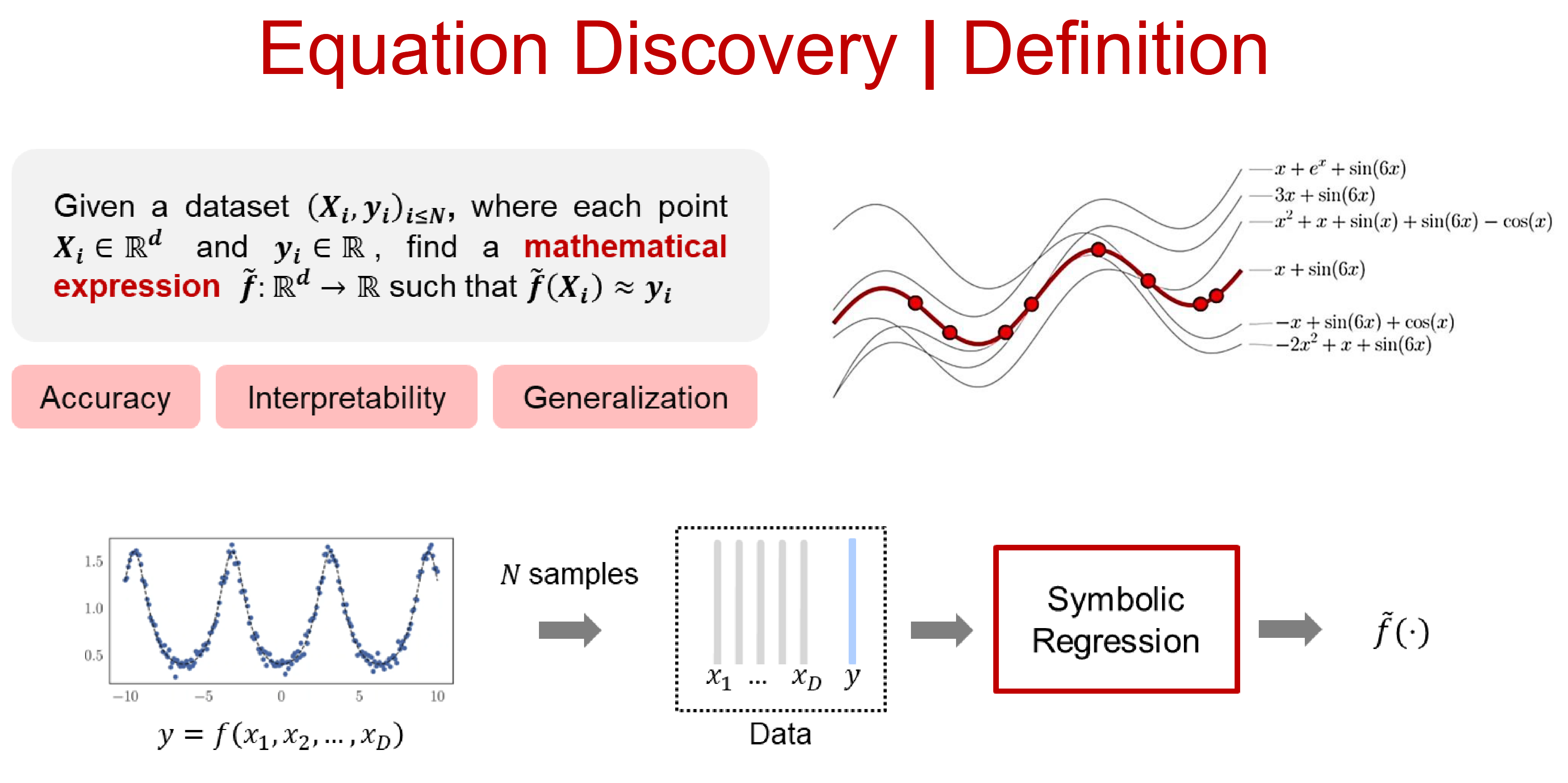
The process of discovering symbolic expressions from experimental data is hard and has traditionally been one of the hallmarks of human intelligence. Symbolic Regression (SR) is a branch of regression analysis that tries to emulate such a process.

More formally, given a set of \(n\) input-output pairs \({(x_i, y_i)}_{i=1}^n \sim \mathcal{X} \times \mathcal{Y}\), the goal is to find a symbolic equation \(e\) and corresponding function \(f_e\) such that \(y \approx f_e(x)\) for all \((x, y) \in \mathcal{X} \times \mathcal{Y}\). In other words, the goal of symbolic regression is to infer both model structure and model parameters in a data-driven fashion.

Even assuming that the vocabulary of primitives — e.g. \({\sin, \exp, +, \ldots}\) — is sufficient to express the correct equation behind the observed data, symbolic regression is a hard problem to tackle. The number of functions associated with a string of symbols grows exponentially with the string length, and the presence of numeric constants further exacerbates its difficulty.

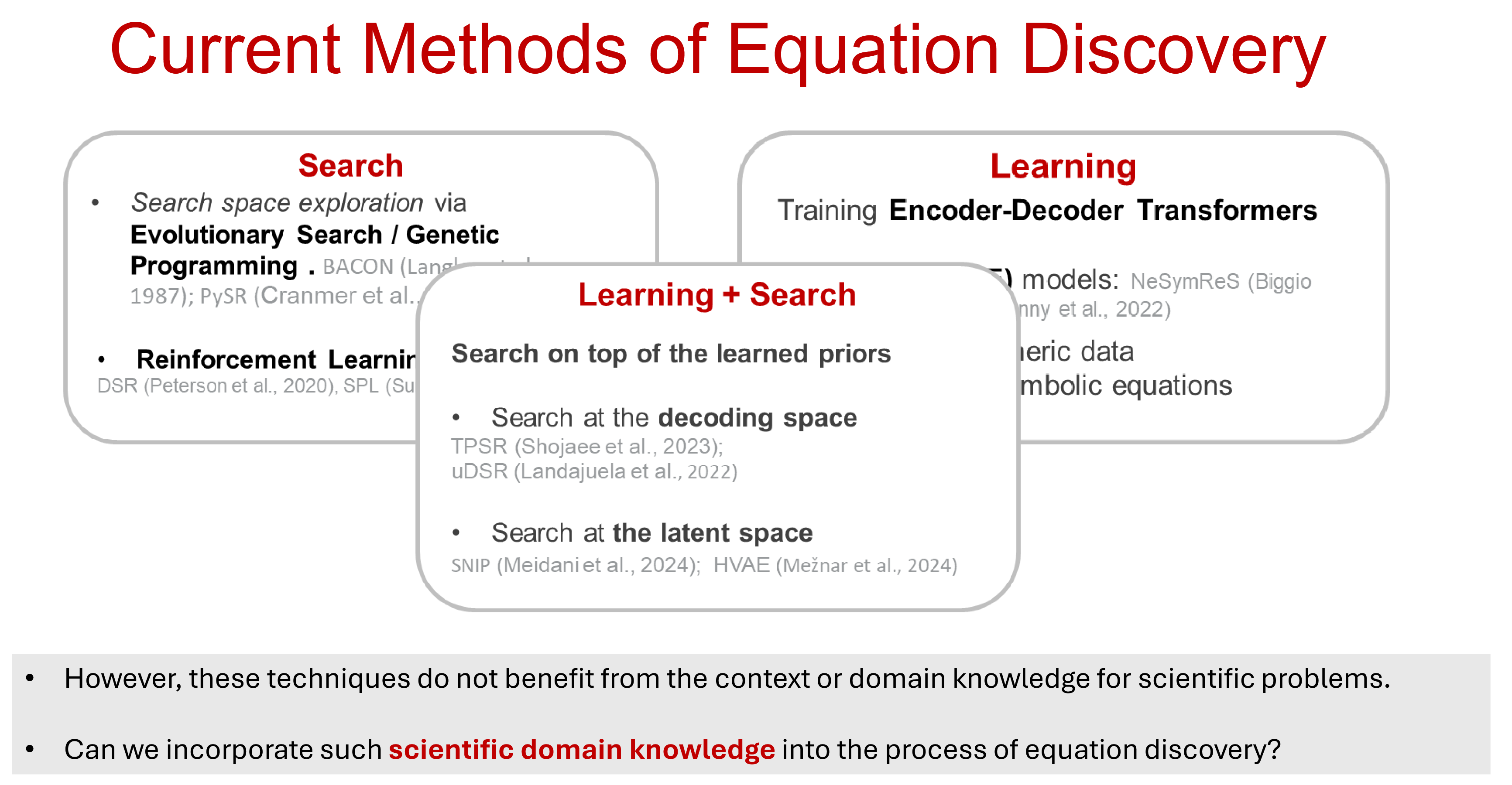
Due to its challenging combinatorial nature, existing approaches to symbolic regression are mainly based on search-techniques whose goal is typically to minimize a prespecified fitness function measuring the distance between the predicted expression and the available data.

To overcome both drawbacks, recent works take a step back and let the model learn the task of symbolic regression over time, on a user-defined prior over equations.

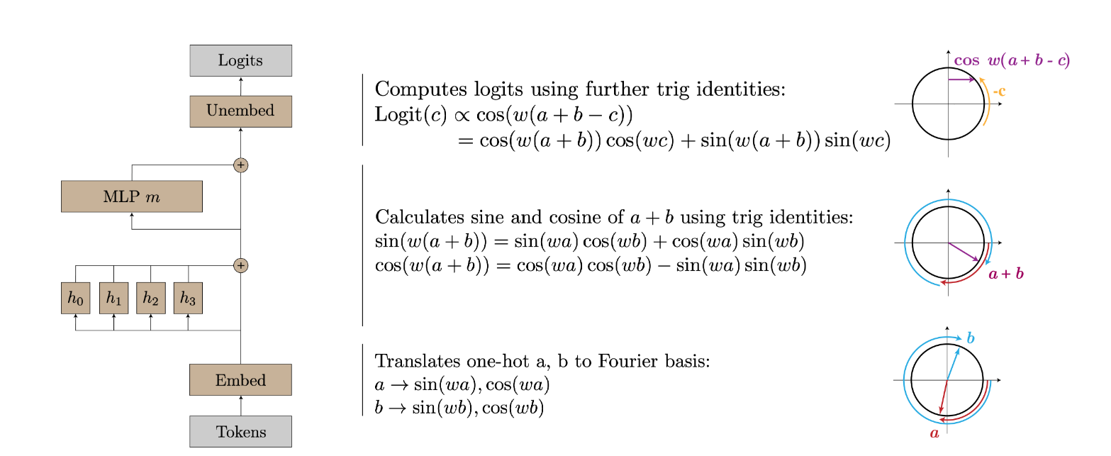
Implicit Math: The “Fourier” Bridge

Before building dedicated SR tools, it’s worth noting that LLMs already perform “implicit” math. Research shows they use Fourier features and trigonometric identities to solve arithmetic tasks [Nanda et al., 2023], essentially learning a spectral algorithm for processing numbers.

The Evolution of SR Methods

The field has shifted from pure search to deep learning, and finally to hybrid approaches. This trajectory mirrors the Bitter Lesson: learned methods that leverage compute scale better than human-engineered heuristics.

1. Search (The Classical Era): Genetic Programming (e.g., Eureqa) searches the equation space directly. While interpretable, it lacks “experience”—solving one problem doesn’t help with the next—and struggles with high dimensions.

2. Learning (The Neural Era): Papers like NeSymReS [Biggio et al., 2021] and End-to-End SR [Kamienny et al., 2022] treat SR as a translation task (Data \(\to\) Equation). By training Transformers on millions of random equations, they learn the grammar of mathematics from data, replacing engineered crossover rules with learned priors.

1. Hybrid & LLMs (The Modern Era): The SOTA now combines the best of both.
   • Guided Search: uDSR [Landajuela et al., 2022] uses neural models to guide genetic search, making it exponentially more efficient.
   • Scientific Priors: EqGPT [Xu et al., 2025] and LLM-SR [Shojaee et al., 2025] use LLMs pre-trained on math/physics handbooks. LLM-SR even treats equations as programs (Python functions), using the LLM to hypothesize structures and standard optimization to fit parameters.

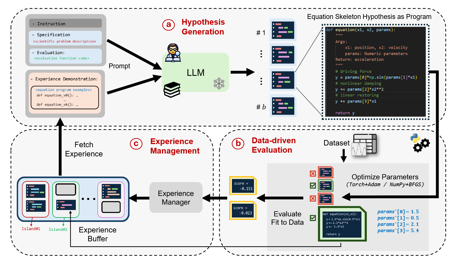
This evolution proves that the ultimate prior is not hand-coded physics, but learned physics—acquired by reading every textbook in the training corpus.

Q4: Are we still suffering from the bitter lessons?

To address this, let’s first summarize The Bitter Lesson by Rich Sutton [Sutton, 2019]:

Computer Vision: From SIFT to AlexNet

An extraordinary real-world example lies in the computer vision community. Before AlexNet won the ImageNet competition in 2012 [Krizhevsky et al., 2012], the field relied on classical methods like SIFT [Lowe, 2004], which used features guided by human experts and prior knowledge. Deep learning proved that this man-made knowledge was not required. If we work with deep neural networks, the primary concerns become model architecture, loss functions, and hardware training. The task transforms completely into an engineering problem.

From Convolutions to Transformers

Following the success of AlexNet, the community explored how to apply deep networks to all kinds of tasks. Traditionally, we used Convolutional Neural Networks (CNNs), which possess an inductive bias inspired by human neuroscience (the receptive field). However, in 2017, the Google team proposed the Transformer [Vaswani et al., 2017], replacing traditional convolution-based modules with self-attention.

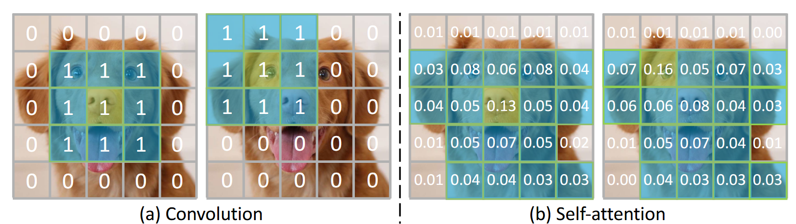
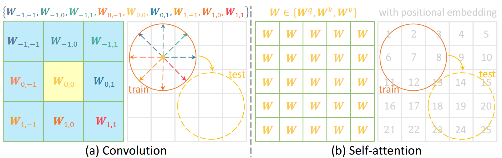
Self-attention is essentially a generalization of the convolutional kernel. This relationship can be formalized mathematically. Let \(\mathcal{C}^{\mathrm{conv}}_{G}\) be the class of translation-equivariant, finite-support Toeplitz operators (convolutional kernels) and \(\mathcal{A}^{\mathrm{attn}}\) the class of self-attention kernels with relative positional structure. We can write:

\[\boxed{ \mathcal{C}^{\mathrm{conv}}_{G}\ \sqsubseteq^{\mathrm{bias}}\ \mathcal{A}^{\mathrm{attn}} }\]

where \(\sqsubseteq^{\mathrm{bias}}\) means “is a constrained instance of (via inductive-bias constraints)”. In plain terms, convolution is a simplified, efficient expression of attention obtained by enforcing fixed translation symmetry, parameter tying, and locality. While convolution can degrade attention to a classic local operator, self-attention generally captures global correlations for each token or pixel, with no predefined locality.

By removing these human-inspired constraints, attention learns which symmetries and long-range relations matter—delivering higher semantic “bandwidth” without a hard-coded translation prior. This inclusion explains why, as data and compute grow, attention-based models have achieved far greater success in vision, language, and robotics, echoing The Bitter Lesson: general methods with fewer hand-engineered priors dominate at scale.

Simplification of Training Recipes

The same “bitter lesson” applies to training recipes and architectures for conditional generation (e.g., vision foundation models). In the early days, researchers designed sophisticated modules to integrate conditional information. Nowadays, the standard recipe is to incorporate the condition at the input level and perform general end-to-end training. Without sophisticated residual designs, these models achieve great success simply by scaling the compute budget.

All this evidence leads us to rethink: Does human knowledge lead us to strong models and AGI, or should we aim to “think like a machine” and prioritize scalable, general methods?

Case Study 1: Generalization via Image Generation Models

An interesting case for generalization in Deep Neural Networks (DNNs) comes from image generation models like Stable Diffusion. We find that models trained on web data are able to generate awesome out-of-domain images, such as ‘a teacher cat in front of a blackboard’, which has likely never been seen during their training stage.

This suggests that the model learns a general manifold of the visual world. Instead of simply memorizing training examples, it captures the underlying structure of concepts (cats, teachers, blackboards) and their relationships, enabling it to synthesize novel combinations that lie on the manifold but were not present in the dataset.

---

Case Study 2: Scientific Discovery via Symbolic Regression

Building on our discussion in Q3 about using deep neural networks for symbolic regression, we now explore a concrete scientific discovery problem: deriving the law of blackbody radiation.

The Scientific Problem

Blackbody radiation describes the electromagnetic radiation emitted by an idealized object that absorbs all incident radiation [OpenStax, 2025]. The key insight is that the intensity of emitted radiation \(I(\lambda, T)\) depends on both the wavelength \(\lambda\) and the temperature \(T\) of the blackbody.

The Symbolic Regression Hypothesis

The core hypothesis is: there exists a compact mathematical equation that describes the relationship between temperature, wavelength, and radiation intensity—rather than a black-box deep neural network.

Historically, this is exactly what happened. Before Planck’s breakthrough in 1900, the Rayleigh-Jeans law attempted to describe this relationship using classical physics but famously failed at short wavelengths (the “ultraviolet catastrophe”). Planck’s revolutionary insight introduced energy quantization, leading to:

\[I(\lambda, T) = \frac{2\pi h c^2}{\lambda^5} \cdot \frac{1}{e^{hc/\lambda k_B T} - 1}\]

where \(h\) is Planck’s constant, \(c\) is the speed of light, and \(k_B\) is Boltzmann’s constant.

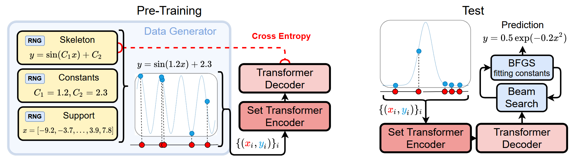
The NeSymReS Approach

Can we rediscover such equations using neural symbolic regression? The Neural Symbolic Regression that Scales (NeSymReS) [Biggio et al., 2021] provides a framework for this task.

The Task Setup:

• Input: Pairs of \((\lambda, T)\) values
• Target Output: Radiation intensity \(I(\lambda, T)\)
• Goal: Discover the mathematical equation connecting them

The key advantage of this approach is that the discovered equation is interpretable and generalizable—it captures the true physical law rather than memorizing training data points. This is the essence of scientific discovery: finding the simplest explanation that accounts for all observations.

---

References

1. Welch Labs (2025). The Most Complex Model We Actually Understand. [YouTube Video].

2. Rumelhart, D. E., Hinton, G. E., & Williams, R. J. (1986). Learning representations by back-propagating errors. Nature, 323(6088), 533-536.

3. Nair, V., & Hinton, G. E. (2010). Rectified Linear Units Improve Restricted Boltzmann Machines. In Proceedings of the 27th International Conference on Machine Learning (ICML) (pp. 807–814).

4. Hendrycks, D., & Gimpel, K. (2016). Gaussian Error Linear Units (GELUs). arXiv preprint arXiv:1606.08415.

5. Klambauer, G., Unterthiner, T., Mayr, A., & Hochreiter, S. (2017). Self-Normalizing Neural Networks. In Advances in Neural Information Processing Systems (NeurIPS) (Vol. 30).

6. Shazeer, N. (2020). GLU Variants Improve Transformer. arXiv preprint arXiv:2002.05202.

7. Li, H., Xu, Z., Taylor, G., Studer, C., & Goldstein, T. (2018). Visualizing the Loss Landscape of Neural Nets. In Advances in Neural Information Processing Systems (Vol. 31). Curran Associates, Inc.

8. He, K., Zhang, X., Ren, S., & Sun, J. (2016). Deep Residual Learning for Image Recognition. In Proceedings of the IEEE Conference on Computer Vision and Pattern Recognition (CVPR).

9. Huang, G., Liu, Z., Weinberger, K. Q., & van der Maaten, L. (2017). Densely connected convolutional networks. In Proceedings of the IEEE Conference on Computer Vision and Pattern Recognition (CVPR).

10. Cortes, C., & Vapnik, V. (1995). Support-Vector Networks. Machine Learning, 20(3), 273–297.

11. Breiman, L. (2001). Random Forests. Machine Learning, 45(1), 5–32.

12. Zhang, C., Bengio, S., Hardt, M., Recht, B., & Vinyals, O. (2017). Understanding Deep Learning Requires Rethinking Generalization. In International Conference on Learning Representations (ICLR).

13. Allen-Zhu, Z., Li, Y., & Song, Z. (2019). A Convergence Theory for Deep Learning via Over-Parameterization. Proceedings of the 36th International Conference on Machine Learning, 242–252.

14. Sutskever, I. (2025). Interviewed by Dwarkesh Patel. We’re moving from the age of scaling to the age of research. The Dwarkesh Podcast. [Podcast].

15. Power, A., Burda, Y., Edwards, H., Babuschkin, I., & Misra, V. (2022). Grokking: Generalization Beyond Overfitting on Small Algorithmic Datasets. arXiv preprint arXiv:2201.02177.

16. Nakkiran, P., Kaplun, G., Bansal, Y., Yang, T., Barak, B., & Sutskever, I. (2020). Deep Double Descent: Where Bigger Models and More Data Hurt. International Conference on Learning Representations (ICLR).

17. Nanda, N., Chan, L., Lieberum, T., Smith, J., & Steinhardt, J. (2023). Progress Measures for Grokking via Mechanistic Interpretability. The Eleventh International Conference on Learning Representations (ICLR).

18. Karpathy, A. (2025). Animals vs Ghosts. [Blog Post].

19. Zhou, T., Fu, D., Sharan, V., & Jia, R. (2024). Pre-Trained Large Language Models Use Fourier Features to Compute Addition. NeurIPS 2024.

20. Nikankin, Y., Reusch, A., Mueller, A., & Belinkov, Y. (2025). Arithmetic Without Algorithms: Language Models Solve Math with a Bag of Heuristics. ICLR 2025.

21. Kantamneni, S., & Tegmark, M. (2025). Language Models Use Trigonometry to Do Addition. Workshop on Reasoning and Planning for LLMs.

22. Ameisen, E., et al. (2025). Circuit Tracing: Revealing Computational Graphs in Language Models. Transformer Circuits Thread. [Blog Post].

23. Gurnee, W., et al. (2025). Attribution Graphs: Methods and Insights from Model-Manifold Geometry. Transformer Circuits Thread. [Blog Post].

24. Biggio, L., Bendinelli, T., Neitz, A., Lucchi, A., & Parascandolo, G. (2021). Neural Symbolic Regression that Scales. Proceedings of the 38th International Conference on Machine Learning, 936–945.

25. Lample, G., & Charton, F. (2020). Deep Learning For Symbolic Mathematics. International Conference on Learning Representations.

26. Kamienny, P.-A., d’Ascoli, S., Lample, G., & Charton, F. (2022). End-to-End Symbolic Regression with Transformers. Advances in Neural Information Processing Systems, 35, 10269–10281.

27. Landajuela, M., Lee, C., Yang, J., Glatt, R., Santiago, C. P., Aravena, I., Mundhenk, T. N., Mulcahy, G., & Petersen, B. K. (2022). A Unified Framework for Deep Symbolic Regression. Advances in Neural Information Processing Systems.

28. Holt, S., Qian, Z., & van der Schaar, M. (2023). Deep Generative Symbolic Regression. The Eleventh International Conference on Learning Representations.

29. Fong, K. S., Wongso, S., & Motani, M. (2023). Rethinking Symbolic Regression: Morphology and Adaptability in the Context of Evolutionary Algorithms. The Eleventh International Conference on Learning Representations.

30. Li, W., Li, W., Yu, L., Wu, M., Sun, L., Liu, J., Li, Y., Wei, S., Deng, Y., & Hao, M. (2024). A Neural-Guided Dynamic Symbolic Network for Exploring Mathematical Expressions from Data. Forty-First International Conference on Machine Learning.

31. Huang, Z., Huang, D. Z., Xiao, T., Ma, D., Ming, Z., Shi, H., & Wen, Y. (2025). Improving Monte Carlo Tree Search for Symbolic Regression. The Thirty-ninth Annual Conference on Neural Information Processing Systems.

32. Xu, H., Chen, Y., Cao, R., Tang, T., Du, M., Li, J., Callaghan, A. H., & Zhang, D. (2025). Generative Discovery of Partial Differential Equations by Learning from Math Handbooks. Nature Communications, 16(1), 10255.

33. Shojaee, P., Meidani, K., Gupta, S., Farimani, A. B., & Reddy, C. K. (2025). LLM-SR: Scientific Equation Discovery via Programming with Large Language Models. The Thirteenth International Conference on Learning Representations.

34. Black Forest Labs. (2025). FLUX.2-dev. [Model Release].

35. Qwen Team (2025). Qwen-Image Technical Report. arXiv preprint arXiv:2508.02324.

36. OpenAI. (2025). New ChatGPT images is here. [Blog Post].

37. Sutton, R. (2019). The Bitter Lesson. [Blog Post].

38. OpenStax. (2025). 6.2: Blackbody Radiation. LibreTexts Physics. [Textbook].

39. Krizhevsky, A., Sutskever, I., & Hinton, G. E. (2012). ImageNet Classification with Deep Convolutional Neural Networks. Advances in Neural Information Processing Systems, 25.

40. Lowe, D. G. (2004). Distinctive Image Features from Scale-Invariant Keypoints. International Journal of Computer Vision, 60(2), 91–110.

41. Vaswani, A., Shazeer, N., Parmar, N., Uszkoreit, J., Jones, L., Gomez, A. N., Kaiser, Ł., & Polosukhin, I. (2017). Attention Is All You Need. Advances in Neural Information Processing Systems, 30.

42. Fan, H., Yang, Y., Kankanhalli, M., & Wu, F. (2025). Translution: Unifying Self-attention and Convolution for Adaptive and Relative Modeling. arXiv preprint arXiv:2510.10060.